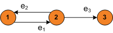
Figure 1: Topology with |N| = 3 nodes, N = {n1,n2,n3}, |E| = 3, E = {e1,e2,e3}. End nodes of e1 are a(e1) = n1
and b(e1) = n2. Outgoing links from node n2 are δ+(n2) = {e2,e3}, and the incoming one is δ-(n2) = {e1}
This guide identifies installation prerequisites, describes how to install Net2Plan, and explains how to run it and extend its functionalities.
Net2Plan is an open-source tool devoted to the optimization and planning of communication networks. The tool is implemented as a MATLAB toolbox together with a Graphical User Interface (GUI).
Net2Plan has been thought as a tool to assist the teaching of communication networks planning courses. It allows testing several built-in algorithms and users (i.e. students) can easily implement and test their own-made algorithms. This process is facilitated by a set of included libraries. The integration of the user-made algorithms in the tool is straightforward. The algorithms are implemented as MATLAB .m files with a mandatory format for input and output parameters. Algorithms in this form can be readily integrated into Net2Plan by simply storing them in the appropriate directory (see section 10).
In Net2Plan a network topology is defined as a graph G(N,E), where N is the set of nodes and E is the set of links. The number of nodes and links are the cardinality of sets N and E, which are |N| and |E|, respectively. Network topologies are considered as multi-digraphs. This means that every link is unidirectional (directed graph or digraph), and that network topologies can have multiple links between the same node pair. No self-links are allowed.
Given a link e ∈ E, a(e) denotes the initial node of the link, and b(e) denotes its destination node. We use l(e) to denote the link length (measured in km). Given a node n, δ+(n) is the set of outgoing links from n (δ+(n) = {e ∈ E : a(e) = n}) and δ-(n) is the set of incoming links to n (δ-(n) = {e ∈ E : b(e) = n}). In Fig. 1 an example of network topology is shown.
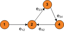
Given a network topology G(N,E), a path p is an ordered sequence of links p = (e1,…,ek), such that the destination node of a link ei is the origin node of the following link ei+1. The set of all possible paths in a network is denoted as P. The first node of the path a(p) is the origin node of the first link a(e1), and the last node in the path b(p) is the destination node of the last link b(ek). Finally, given a link e ∈ E, Pe is the set of paths which traverse the link e. For example in Fig. 2, given p1 = {e12,e23,e34} and p2 = {e42,e23}, Pe23 = {p1,p2}. In addition, l(p) is the number of hops in path p.
An important concept in networks is the so-called connectivity. A network is connected if it is possible to find a path from every node to each other. For example, the topology in Fig. 1 is not connected since nodes 1 and 2 are not reachable from node 3. In its turn, the topology in Fig. 2 is connected.
Each node e in a network has associated a real number ue ≥ 0 which represents its capacity. The capacity is the amount of traffic the link is able to carry. Thus, capacities and traffics are measured in the same units. Unless stated otherwise, the traffic and capacities in Net2Plan are measured in Erlangs.
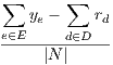
For the sake of simplicity, we denote the set of link capacities as a vector u = {ue,e ∈ E}. In addition, the carried traffic by link e is denoted by ye. The vector y = {ye,e ∈ E} represents the traffic carried in all the links in the network.
Typically link capacities are limited to a discrete range of values due to technological reasons, such as STM-N carriers in SDH. In these cases, capacities are referred as modular capacities.
Traffic is modelled through a set of demands (or commodities) D. Each demand d ∈ D represents an offered traffic flow to the network. In general, a the traffic of a demand d can have one or more ingress nodes in the set a(d), and one or more egress nodes denoted by the set b(d); however, in current version of Net2Plan demands are considered unicast. This means that each demand d has one ingress node and oner egress node, thus |a(d)| = |b(d)| = 1. In addition, self-demands are not allowed.
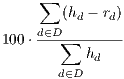
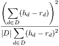
The offered traffic by a demand d is represented as hd. Such value is measured in the same units as link capacities u (i.e. Erlangs). In some situations, it is not possible to carry all the offered traffic by the demands. Then, rd ≤ hd represents the amount of traffic belonging to demand d that is carried. In their vector form, h = {hd,d ∈ D} and r = {rd,d ∈ D} represent offered and carried traffic, respectively.
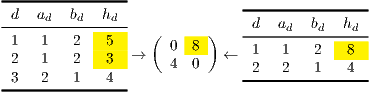
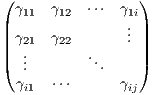
A simplified approach to model the offered traffic between nodes is the so-called traffic matrix. A traffic matrix is a |N|x|N| matrix (where |N| is the number of nodes in the network) in which each pair (i,j) represents the traffic from node i to node j.
The main drawback of representing the offered traffic by means of traffic matrices, is that the traffic matrix representation assumes that at most one demand exists between each pair of nodes. Then, if we compute the traffic matrix representation of a demand set D where some node pairs have more than one demand between them, an ambiguity can occur. This situation is posed in Fig. 3, where demands 1 and 2 from the demand set on the left are grouped in a single entry in the traffic matrix. The same result is obtained with the demand set on the right.
Routing is the process of selecting paths in a network along which to send the traffic. In Net2Plan, the routing is represented in the form of demand-path variables. As stated in section 3.1, where paths were defined as sequences of links from a origin node to a destination node, a path for a demand is defined as a path from the ingress node to the egress node of that demand.
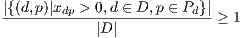
Formally, for each demand d in the network, a set of paths Pd ⊂ P is defined between the end nodes of the demand (a(d) = a(p),b(d) = b(p)). Then, traffic routing is represented by a vector:
| x = {xdp,d ∈ D,p ∈ Pd} |
Next, two typical routing constraints are described:
Table 1 summarizes information about background underlying Net2Plan.
| Element | Parameter | Description |
| Nodes | N | Set of nodes n ∈ N |
| δ+(n), δ-(n) | Set of outgoing and incoming links from/to node n | |
| Links | E | Set of links e ∈ E |
| a(e), b(e) | Origin and destination nodes of link e | |
| le | Length of link e (Km) | |
| ue | Capacity of link e (Erlangs) | |
| u | Vector form of ue | |
| ye | Traffic carried by link e (Erlangs) | |
| y | Vector form of ye | |
| All links are considered unidirectional
| ||
| Self-links are not allowed (a(e)≠b(e))
| ||
| Paths | P | Set of all possible paths in the network p ∈ P |
| Pe | Subset of the paths in P that traverse link e | |
| p = {…} | Sequence of links traversed in path p | |
| a(p), b(p) | Origin and destination nodes of path p | |
| l(p) | Number of hops in path p | |
| Demands | D | Set of demands d ∈ D |
| a(d), b(d) | Ingress and egress nodes of demand d | |
| hd | Offered traffic for demand d (Erlangs) | |
| h | Vector form of hd | |
| rd | Carried traffic for demand d (Erlangs) | |
| r | Vector form of rd | |
| Pd ⊂ P | Set of valid paths defined to carry traffic from demand d (a(d) = a(d) and b(p) = b(d)) | |
| Demands are unicast
| ||
| Self-demands are not allowed (a(d)≠b(d))
| ||
| Pde | Set of valid paths for d that traverse e (a(d) = a(d) and b(p) = b(d)) | |
| Routing | xdp | Fraction of hd carried by p ∈ Pd |
| x | Vector form of xdp | |
In practical network design different variables can be involved: link capacities, the traffic routing, the topological design of the network, the storage capacity at each node, and so on. Usually, network design problems receive some of this information as input parameters (e.g. traffic demand, and network topology) and try optimize the rest (e.g. capacities in the links and traffic routing) according to a performance merit of interest. Clearly, the number of possible variants and subtypes of network design problems is infinite. Moreover, different technologies add their own particular aspects to network design. For this reason, network design has become a mixture of art and engineering.
In an attempt to provide a (somehow) systematic criteria to cathegorize network design problems, in Net2Plan we adopted the following scheme, which is just an extension of the network design problems’ taxonomy in Kleinrock’s book [1]:
According to this naming scheme, combinations of these problems are named combining the acronyms. For example, a capacity and flow assignment (CFA) problem involves the joint computation of routing and link capacities. We remark that this taxonomy should be considered as an attempt to give a didactic organization to the utmost diversity of planning problems that arise in communication networks.
Typically network design problems are presented as optimization problems, this means that there are a set of performance criteria to maximize or minimize, subject to some constraints (qualitative statements about network design and performance), given a set of input parameters (i.e. partial network designs). Optimization algorithms (or just “algorithms”) are the methods that compute a numerical solution to a given problem instance. In Net2Plan, an algorithm is a .m file with a given signature (see section 8 for more information) that fix the format of the input and output parameters.
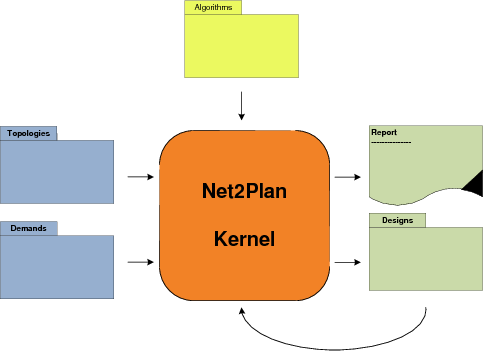
Net2Plan is divided into two main parts: graphical user interface (GUI) and kernel. The main idea is that all the design algorithms, independently of their specific target, receive as input parameter the current network structure (see section 4.2), and return an updated version of this network structure. Then, the Net2Plan kernel and GUI, are devoted to just process the designs returned by the algorithms: check its validity (e.g. the topology has a correct format, the links are not oversubscribed etc), graphically display the network design, and compute some reports and performance merits.
The idea behind Net2Plan is that you can progressively design your network. This is, you can chain successive algorithms, each one completing a part of the network design. For instance, you can start with a network where only the nodes are defined. Then, an algorithm is used to define the links in the network according to some figure of performance. Afterwards, an algorithm can be run to jointly decide on the capacity in the links and routing of the flows, for a given traffic matrix. As a result, Net2Plan can be a powerful tool for communications network planning courses, since students can see step by step how their designs grow.
Net2Plan assists the task of creating and evaulating network design algorithms by providing built-in example algorithms. In section 10, a list of built-in algorithms can be found. In section 8 we explain in more detail how to integrate new algorithms in Net2Plan.
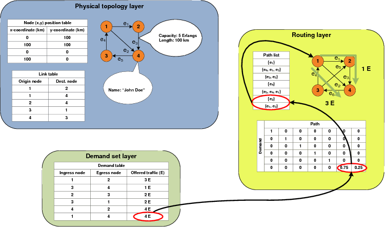
In Net2Plan, data files are stored as .xml files containing all kind of information: network topology, traffic demands, routing, and so on. This information is organized in a hierarchy of layers:
Physical topology layer contains (X,Y )-coordinates of nodes, their names and a set of optional and user-defined attributes per each node. In addition, it contains origin and destination node of each link, its length and capacity, and also a set of optional per-link attributes.
Demand set layer contains ingress and egress nodes, average offered and carried traffic volume and a set of optional and user-defined attributes per demand. It contains information about carried traffic, if routing layer information is available.
Routing layer contains a set of paths to carry traffic from demands across the network. Each path is represented by the set of links traversed in that path. In addition, it contains a routing matrix which shows how traffic demands are carried over the paths.
Fig. 5 shows an example of complete network design including all items stated previously.
In order to use this information within Net2Plan, a structure called netStruct is created with the following fields:
As a convention, every user-defined attribute is assumed to be a string. Algorithms must check these attributes and convert them to the appropriate type, in case they use them.
According to the network depicted in Fig. 5, netStruct would be as follows:
Finally the mapping of the previous netStruct on .xml file is shown:
To install Net2Plan, save the compressed file in any directory. Then, extract all the files and folders into a new directory, for example, C:\Work\Net2Plan.
To run Net2Plan, start MATLAB, change current directory to the installation directory, and run startup.
Net2Plan requires MATLAB 7.9.0 (R2009b) or higher versions and a screen resolution of, at least, 800x600 pixels.
In order to start the Net2Plan tool, execute MATLAB, change the current directory to \Net2Plan and execute startup.m. As a result, the welcome screen will be shown. If you want to use CVX solver you must initialize it using the appropriate CVX command, before executing Net2Plan.
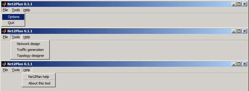
In the top menu you can choose between the different options which Net2Plan provides. Below are listed and explained:
This menu has two items: Options and Quit.
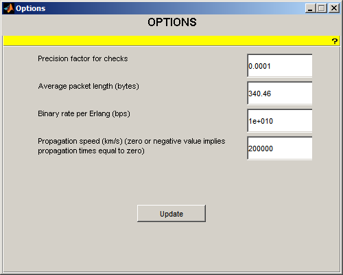
Use Options to set Net2Plan-wide parameters. These options have a global scope to all Net2Plan modules: are used within the kernel, and to compute delay metrics, for example. In this version there are only four options:
Options are saved when you press “Update” button. Then new values are checked and saved in the options file.
Use Quit to close Net2Plan.
This menu has three items: Network design, Traffic generation and Topology designer.
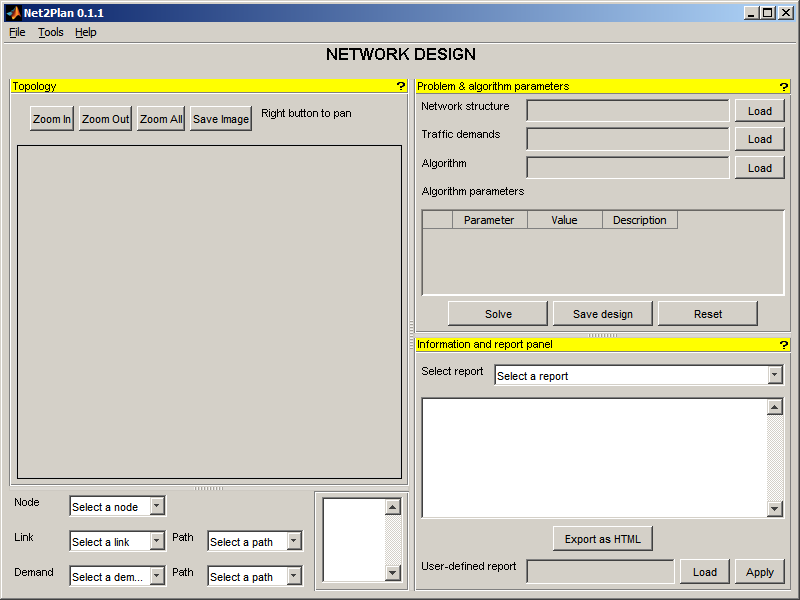
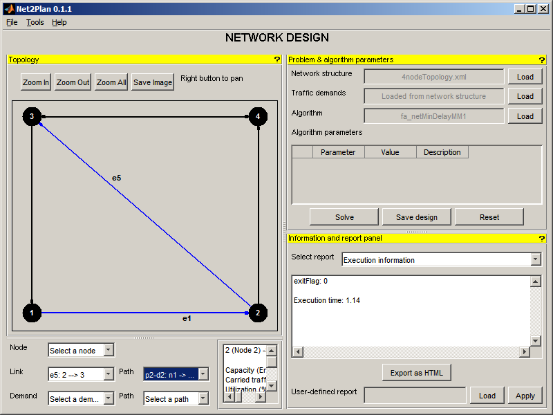
Selecting Network design opens the Network design window, which you can use to execute your algorithms.
The workspace of the window is divided into three areas: input data (top-right area), plot area (left), and results report area (bottom-right area).
Problem & algorithm parameters The user should define the input parameters for the execution in the input area. In general, to calculate a new design the user has to specify the following things:
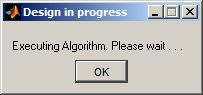
Once those inputs are filled, the algorithm can be executed by clicking on “Solve”. A popup will be shown during the execution of the algorithms (see Fig. 10). When the execution finishes, a message will be shown, informing if the algorithm run well (see Fig. 11) or some error was thrown (see Fig. 12).
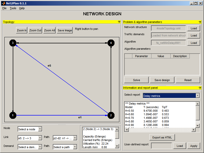
Topology In this panel you can see the current state of the network design. If the design includes routing information, it is possible to visualize the paths which carry traffic of a demand, the paths traversing a link,... In addition, a small box shows brief information about the item selected in the topology (node, link, demand, path).
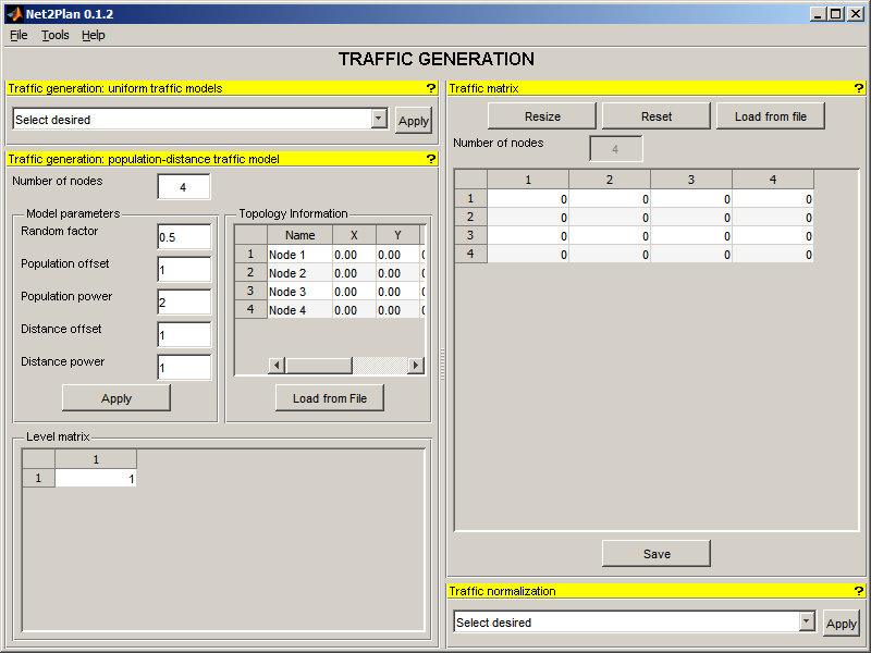
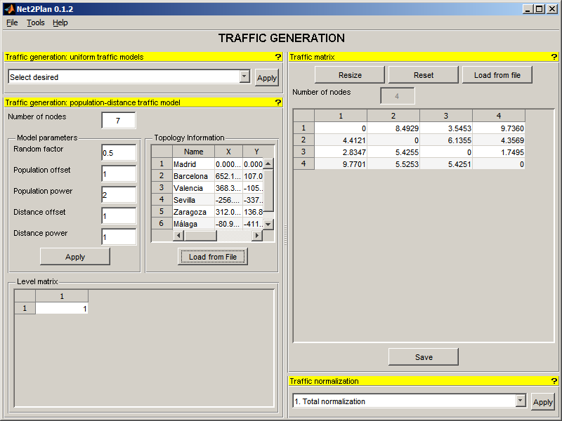
Selecting Traffic generation under Tools menu activates the Traffic generation window. This interface allows the user to generate a .xml file representing a traffic matrix. This figure displays the workspace window for this option.
The Traffic generation window is divided into four different parts:
Traffic matrix The user initiates the process by selecting the number of nodes N in the network using Resize option. The traffic matrix will be like this:
 | (1) |
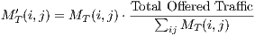 | (2) |
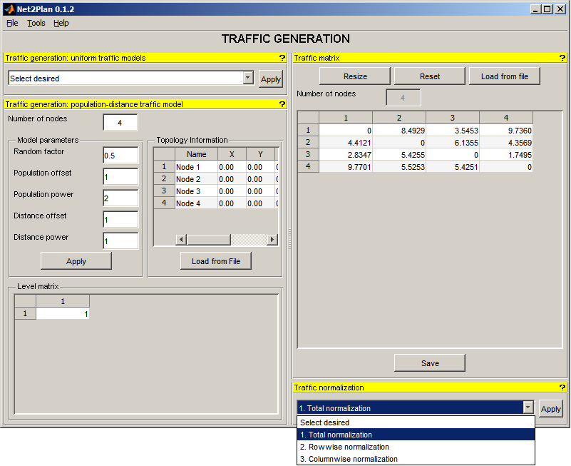
where MT′ is the normalized traffic matrix and MT is the original traffic matrix.
The user introduces the total offered traffic volume in a popup.
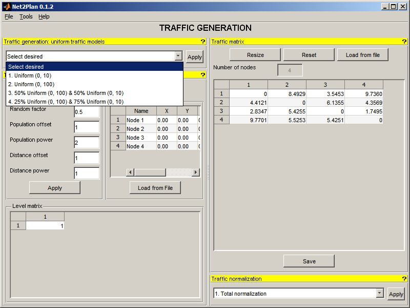
Traffic generation: uniform traffic models After this, the user can select one of the traffic generation patterns among the five modes available: four of them are simpler, and based on the uniform distribution.
Please note at the end of this process diagonal values of traffic matrix are zero, since self-demands are not allowed.
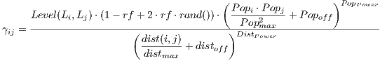
Traffic generation: population-distance traffic model The fifth mode allows creating a traffic matrix according to the model described in [2]. This latter model applies the information of node position, population and node level, present in a topology information table (user can load a topology from a .xml file). The distribution based on populations and distances follows the next expression:
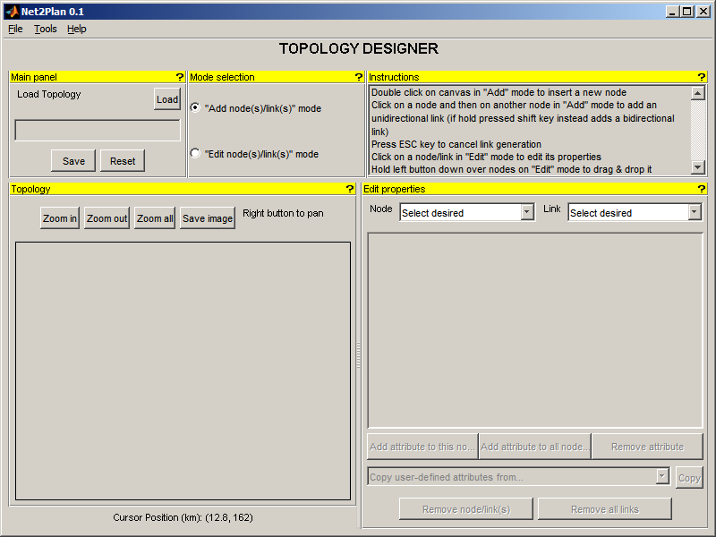
where Level is a L×L two-dimensional matrix (L: number of levels or node types defined by the user). This matrix allows us to introduce asymmetric traffic in the traffic generator; Popi is the population of the node i; Popmax is the maximum population; dist is a matrix N × N (N: number of nodes) with the distances between nodes; distmax is the maximum distance.Selecting Topology designer under Tools menu activates the Topology designer window. This interface allows the user to generate a .xml file representing a network topology. This figure displays the workspace window for this option.
Main panel Here you can load and save network designs.
Mode selection Here you can change the mode of the tool. In “Add mode” you can add nodes and links, and in “Edit”
mode you can edit them.
Instructions Here instructions to design topologies are shown. In sections below are reproduced.
Topology This panel is used for graphically design networks. It is very similar to the topology panel in the network
design tool, but it has certain new functionalities.
Nodes are inserted by double clicking into the canvas with the “Add” mode activated.
Links are inserted by clicking first in the origin node and then in the destination node. It is possible to insert unidirectional
links or bidirectional ones (in this case, you must press SHIFT key during that process).
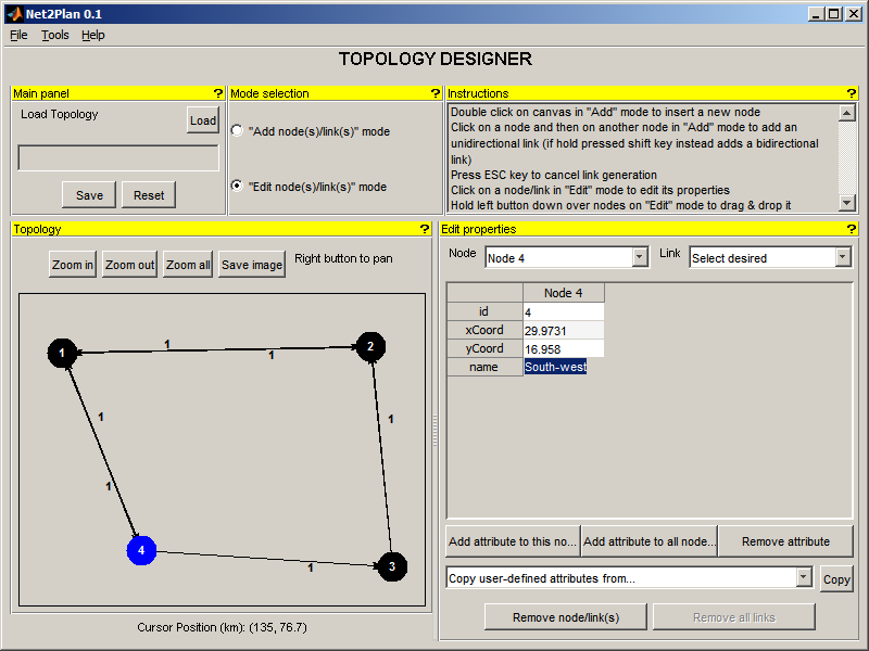
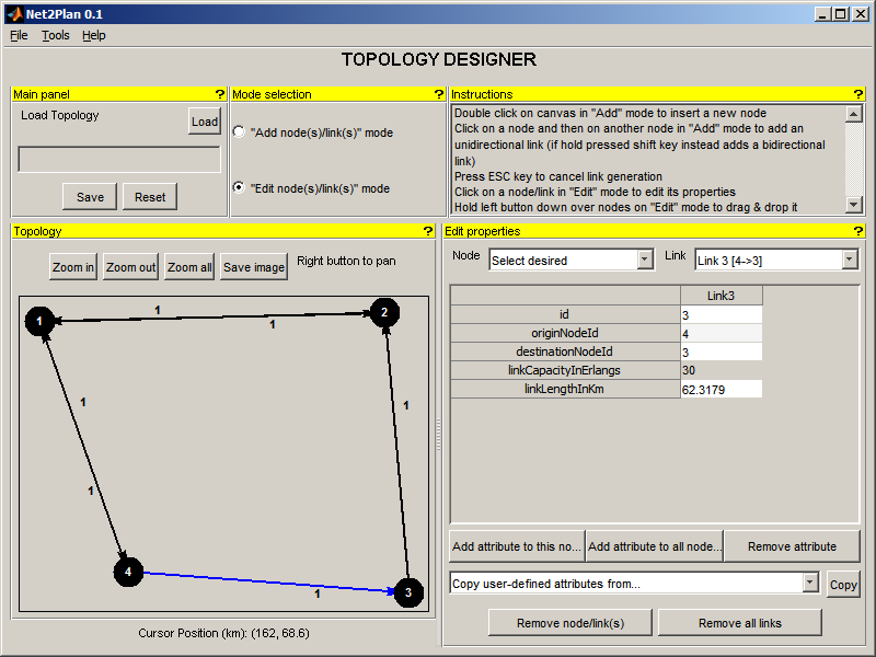
Edit properties When you have nodes and links placed, you can edit their properties by clicking on them with the
“Edit” mode activated. Not all properties can be changed, i.e. “Node Identifier” is generated internally. The following
figures show two examples.
This menu has two items: Net2Plan help and About this tool.
You can read this file.
It shows the welcome screen.
This section describes the directory structure in the toolbox. It has the following folders:
| Directory | Description |
| \algorithms | Includes built-in algorithms. User-made algorithms must be placed here |
| \data | Includes topologies, traffic matrices and result files. User-made designs can be placed here |
| \help | Includes help file |
| \kernel | Includes kernel of the tool. It is recommended not to modify any file here |
| \libraries | Includes auxiliary libraries to develop algorithms |
| \userDefinedReports | Includes user-defined reports. User-made reports must be placed here |
New algorithms can be implemented as MATLAB functions (.m files) with a given signature. Integration of algorithms simply requires saving them in any directory of the computer, although it is a good practice to store them in \algorithms directory.
The signature must be like this:
[exitFlag, exitMsg, netStruct] = algorithmName (netStruct, algorithmParameters, net2planParameters)
The input parameters are defined as follows:
The output parameters are:
The task of generating new network design algorithms in Net2Plan, is facilitated by a set of built-in libraries included (see section 11).
When creating a new algorithm, the developer can specify a set of input parameters to tune the algorithm functionality. The kernel recognizes that the algorithm has input parameters
To declare the input paramters of an algorithm to the kernel, the .m implementnig the algorithm must include in the help text of the file, one line per parameter in the format:
When the Net2Plan user selects an algorithm, the kernel processes the help string of the .m file, and obtains the input parameters to the algorithm, their default values, and a description string that is displayed in the GUI to inform the user. When the user clicks the solve button, the kernel passes to the algorithm the algorithmParameters structure. In this structure, each parameter is passed to the algorithm as a char. The algorithm implementation should perform the appropriate conversions to the specific type, making any sanity checks if needed. For example, the next snippet shows how to define a new algorithm with two parameters and how to convert the input parameters to a numerical format.
In addition to reports generated by Net2Plan user can define reports which returns every kind of information that user requires.
As stated for algorithms, user-defined reports can be implemented as MATLAB functions with a given signature. Integration of user-defined reports simply requires saving them in any directory of the computer, although it is a good practice to store them in \userDefinedReports directory.
The signature must be like this:
msg = functionName(netStruct, net2planParameters)
Input parameters are structures defined according to sections 4.2 and 6.1.1, and the output parameter must be a string. User is responsible to validity of these reports and to check netStruct prior to their computation.
Next, an example of user-defined report is shown:
In this section we enumerate all the algorithms included in Net2Plan distribution. These algorithms are organized in folders according to the problem type they address.
| Family | Algorithm | Description |
| Bandwidth assignment | ba_networkUtilityMaximization | Solve the Network Utility Maximization (NUM) problem giving an alpha-fair bandwidth for traffic demands. Require CVX solver installed and running |
| Capacity assignment | ca_fixValue | Set a constant capacity value for all links |
| ca_minAvDelayConcaveCost | Minimizes the average network delay, with concave cost constraints. Requires CVX solver installed and running | |
| ca_minAvNetDelayLinearCost | Minimizes the average network delay, with linear cost constraints. Requires CVX solver installed and running | |
| ca_netMinimaxUtilization | Minimizes the maximum link utilization, with linear cost constraints. Requires CVX solver installed and running | |
| Capacity and flow assignment | cfa_shortestPathInKmFixedUtilization | Shortest path routing and then set the capacities to match a given link utilization |
| Flow assignment | fa_minimaxUtilization_xde | Minimizes the maximum link utilization, using flow-link formulation. Requires CVX solver installed and running |
| fa_minimaxUtilization_xdp | Minimizes the maximum link utilization, using flow-path formulation. Requires CVX solver installed and running | |
| fa_minNetDelay_xde | Minimizes the average network delay, using flow-link formulation. Requires CVX solver installed and running | |
| fa_shortestPath_km | Route all the traffic in the shortest path using link length (km) as the cost figure | |
| fa_shortestPath_numHops | Routes all the traffic in the shortest path using 1 as cost per link | |
| Topology assignment | la_bidirectionalMinimumSpanningTree_Prim_Km | Generates a bidirectional minimum spanning tree using Prim’s algorithm and link length as cost per link |
| la_randomBidirectionalUntilConnected | Randomly generates bidirectional links until the network becomes connected | |
| la_randomUnidirectionalUntilConnected | Randomly generates unidirectional links until the network becomes connected | |
| la_tspNearestNeighbourKmBidirectional | Generates a ring topology using nearest neighbour algorithm with cost of a link given by the link length in km | |
| la_unidirectionalMinimumSpanningTree_Prim_Km | Generates a unidirectional minimum spanning tree using Prim’s algorithm and link length as cost per link | |
| na_randomUniform | Returns a set of nodes randomly placed within a given grid | |
| na_topFiveSpain | Returns a set of nodes (along with a ”population” attribute) representing the five largest cities in Spain (in terms of population) | |
| na_topSevenSpain | Returns a set of nodes (along with a ”population” attribute) representing the seven largest cities in Spain (in terms of population) | |
In this section are shown all libraries included within Net2Plan. These libraries are organized in folders according to the function performed.
| Family | Library | Description |
| checks | isBidirectional | Check if the topology is bidirectional: same number of links between each node pair in both directions (assuming multi-digraphs) |
| isBidirectionalAndSymmetric | Check if the topology is bidirectional and symmetric: same number of links between each node pair in both directions (assuming multi-digraphs) and same weights per direction. Can be used to check if links are bidirectional and distance-symmetric (if weight is link length), bidirectional and capacity-symmetric (if weight is link capacity), if demands are symmetric (if linkTable is demandTable and weight is offeredTrafficInErlangs) and so on | |
| isConnected | Check if the topology is connected | |
| isDemandTable | Check whether a demand table is valid | |
| isLinkTable | Check whether a link table is valid | |
| isPathList | Check whether a path list is valid | |
| isSimpleGraph | Check if a graph is simple: no more than one link per node pair | |
| isTrafficMatrix | Check whether a traffic matrix is valid | |
| computeGraph | floydAlgorithm | Floyd’s algorithm for finding all-pairs shortest path in a weighted graph with positive weights |
| primAlgorithm | Function to generate a minimum spanning tree using Prim’s algorithm | |
| shortestPath | Dijkstra’s algorithm for finding the shortest path between two given nodes | |
| conversions | adjacencyMatrix2linkTable | Function to convert a |N|×|N| adjacency matrix into a |E|× 2 link table where each row represents the origin and destination nodes of the link |
| demandTable2trafficMatrix | Function to convert a |D|× 2 demand table in a |N|×|N| traffic matrix where each entry (i,j) represents the units of traffic from i to j | |
| linkTable2adjacencyMatrix | Compute the adjacency matrix from a link table of a multi-digraph | |
| linkTable2adjacencyMatrix | Compute the incidence matrix from a link table of a multi-digraph | |
| nodeXYPositionTable2distanceMatrix | Compute distance matrix between each node pair from a XY-position table of the nodes | |
| seqLinksPerPath2linkOccupancyPerPath | Function to convert a pathList into a |P|×|E| matrix in which each entry (p,e) represents how many times p traverses link e | |
| sequenceOfLinks2sequenceOfNodes | Given a linkTable and a sequenceOfLinks, return the sequenceOfNodes traversed | |
| sequenceOfNodes2sequenceOfLinks | Given a linkTable and a sequenceOfNodes, return the sequenceOfLinks traversed | |
| trafficMatrix2demandTable | Function to convert a |N|×|N| traffic matrix in a |D|×|2| demand table and |1|×|D| demand vector where the i-th row in demandTable contains the input and output nodes of the demand, and the i-th value in demandVector is the corresponding amount of traffic in Erlangs | |
| xde2xdp | Function to convert from node-link routing to link-path routing | |
| xdp2xde | Function to convert from link-path routing to node-link routing | |
| metrics | erlangBLossProbability | Erlang-B probability of call blocking in a M/M/n/n queue system |
| inverseErlangB | Return ”numberOfServers” required to guarantee a certain ”gradeOfService” under an utilization ”load” in a M/M/n/n queue system | |
| misc | isCvxInstalledAndRunning | Check whether CVX solver is installed and running |
| isSedumiInstalledAndRunning | Check whether SeDuMi solver is installed and running | |
| isYalmipInstalledAndRunning | Check whether YALMIP solver is installed and running | |
| removeRoutingInformation | Function to remove routing information from netStruct when due to any operation (as a link capacity change), it becomes obsolete | |
| trafficPerLink | Function to compute carried traffic per link using a link-path formulation | |
Net2Plan tool has its origins in 2011, during the preparation of the teaching materials for two new Communication Networks Planning courses at Universidad Politécnica de Cartagena (Spain) taught by Prof. Pablo Pavón Mariño:
Net2Plan is also a part of the Ph.D. work of José Luis Izquierdo Zaragoza, supervised by Prof. Pablo Pavón Mariño.
Aside from Net2Plan, authors also collaborate in the development of MatPlanWDM, an open-source tool for multilayer optical networks.
Pablo Pavón Mariño
José Luis Izquierdo Zaragoza
The development of Net2Plan is to a large degree driven by users’ bug reports. In most cases, when providing feedback, it is essential to include the following information:
By the way, please don’t contact authors for doing your assignments or requesting new features, probably you won’t get an answer.
[1] L. Kleinrock, Queueing Systems, Volume 2: Computer Applications. John Wiley & Sons, 1976.
[2] R. S. Cahn, Wide Area Network Design: Concepts and Tools for Optimization. The Morgan Kaufmann Series in Networking, Morgan Kaufmann, 1 ed., July 1998.
[3] P. Pavon-Marino, “Lectures of the Telecommunication Networks Theory course,” 2012.
[4] M. C. Grant and S. Boyd, “CVX: Matlab Software for Disciplined Convex Programming.” Website: http://cvxr.com/cvx/ [Last accessed: January 10, 2012].
Net2Plan 0.1.8 (June 18, 2012)
Net2Plan 0.1.7 (June 4, 2012)
Net2Plan 0.1.6 (May 15, 2012)
Net2Plan 0.1.5 (May 11, 2012)
Net2Plan 0.1.4 (April 18, 2012)
Net2Plan 0.1.3 (April 12, 2012)
Net2Plan 0.1.2 (March 28, 2012)
Net2Plan 0.1.1 (March 16, 2012)
Net2Plan 0.1 (February 2012)
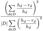
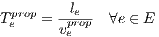
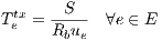
In this section several performance and cost metrics are described. These metrics are useful to define objective functions or problem constraints. For a complete reference on network metrics, see [3].
 | (4) |
 | (5) |
 | (6) |
 | (7) |
 | (8) |
 | (9) |
 | (10) |
 | (11) |
 | (12) |
 | (13) |
 | (14) |
 | (15) |
 | (16) |
 | (17) |
 | (18) |
 | (19) |
![( )
∑ ∑ [∑ ]
rd( xdp le )
d∈D p∈Pd e∈p
---------∑-------------
rd
d∈D](manual21x.png) | (20) |
 | (21) |
 | (22) |
 | (23) |
 | (24) |
 | (25) |
 | (26) |
 | (27) |
In packet-switched networks, traffic sources split data into smaller pieces called packets, along with a header with control information. Per each received packet, switching nodes read its header and take appropriate forwarding decisions.
In real networks, traffic is highly unpredictable and often modelled as random processes. When it is said that a traffic source d generates hd traffic units, it is referred as average traffic. As a result, link capacities would be not enough to forward traffic and nodes have to store packets in queues, so they are delayed until they can be transmitted (this delay is known as queueing delay). If this situation remains for a long time, queues are filled and links become saturated, provoking packet drops.
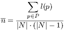
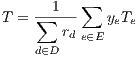
Network design tries to model statistically delays and drops in order to minimize their effects. In Net2Plan each link is modelled as a queue fed by a self-similar source with a given Hurst parameter, getting the whole network average delay using Kleinrock’s independence assumption.
 | (28) |
 | (29) |
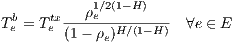 | (30) |
where H ≜ Hurst Parameter (here H doesn’t mean total offered traffic). Choosing H = 0.5 yields to same result predicted by M/M/1 queue model.
 | (31) |
 | (32) |
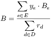
In circuit-switched networks, traffic sources reserve a given capacity during certain time, along paths followed by traffic demands. It is possible that if a new traffic source wants to reserve resources its petition would be blocked, since it would not be enough available resources to satisfy its demand.
Blocking performance metrics are computed using Erlang-B formula. Obviously only has sense when u is integer.
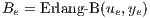 | (33) |
 | (34) |
 | (35) |
CVX is a MATLAB-based modelling system for convex optimization. CVX turns Matlab into a modelling language, allowing constraints and objectives to be specified using standard Matlab expression syntax.
CVX has been used in Net2Plan to develop some algorithms, not in kernel, thus you are free to install or not this solver. Please note that if CVX is not properly installed, algorithms which use it won’t work (take a look into section 10 to see algorithms that use it).
CVX is not shipped with Net2Plan, but it is publicly (and no-charge) available on its website [4]. Once you download CVX (if you decided to use it), you must run cvx_setup in MATLAB to install it.
Net2Plan team don’t provide any support to CVX.